
Before we dig into understanding normal distribution, we should first take a look at what distribution is?
What is distribution?
Distribution is a function that describes how the values of a variable are spread throughout the dataset. It reveals the possibility or frequency of each possible value occurring.
For example, Imagine measuring the heights of 100 people. A distribution tells you that how many people fall within each height range (e.g. 150-155 cm, 155-160 cm, etc.) This helps visualize the spread of heights within the group and estimate the probability of encountering individuals of certain heights.
What is Probability Distribution?
Probability distribution is also known as theoretical frequency distribution and can be defined as distribution of frequencies which is not based on actual experiments or observations but is constructed by mathematical computation based on certain hypothesis.
What is normal distribution?
Normal distribution is a continuous probability distribution that is characterized by its bell-shaped curve. This describes data where most values cluster around the average (center) and become less frequent as they move away from center, and very few data points are extremely far from the average. This bell-shaped curve helps us understand how data is spread out and estimate the probability of encountering specific values within the dataset. s Normal distribution is also known as Gaussian distribution.
What are the features of a normal distribution?
There are several features of normal distribution.
Bell Shaped Curve
Bell shaped curve is the most recognizable feature of normal distribution, the curve shows peak at the center, representing the most frequent values, and tails that taper off gradually towards both ends, indicating lower frequency of extreme values.
Symmetry
The distribution is identical on both side of the mean or we can say the distribution is perfectly symmetrical around the mean (average). This shows that probability of a datapoint appearing a certain distance above the mean is identical to the probability of the same data point appearing at the same distance below the mean.
Mean, Medial, and Mode
The three measures of central tendency are identical in normal distribution, meaning that they fall at the center of curve.
Defined by Two parameters
The normal distribution is fully described by two parameters:
- Mean (μ): This represents the center of the distribution, where the peak of the curve occurs.
- Standard Deviation (σ): This measures the spread of the data points around the mean. A bigger standard deviation shows a wider spread of data points, while a smaller standard deviation shows a tighter clustering around the mean.
Empirical Rule (68-95-99.7 Rule)
This rule states that in a normal distribution:
- Approximately 68% of the data points fall within 1 standard deviation of the mean.
- Approximately 95% of the data points fall within 2 standard deviations of the mean.
- Approximately 99.7% of the data points fall within 3 standard deviations of the mean.
Asymptotic tails
Asymptotic tails represent those two ends of the bell-shaped curve that gradually approach, but never touch, the x-axis.
Z-Score
Distance from mean (μ) to a point (x) in normal distribution is represented by Z-Score.
Vishal Jaiswal, CuriousClub.in
Z score is a method to represent the distance between a specific value and mean. In other words, Z score tells you how many standard deviations(σ) away a point is in a normal distribution. It is calculated with below formula.
Z = (X - μ) / σ
Where:
- X is the specific data point you’re interested in.
- μ is the mean of the normal distribution.
- σ is the standard deviation of the normal distribution.
Interpretation:
- A positive Z score indicates that the data point (X) is above the mean.
- A negative Z score indicates that the data point (X) is below the mean.
- A Z score of 0 means the data point is exactly at the mean.
Let us understand normal distribution with an example below.
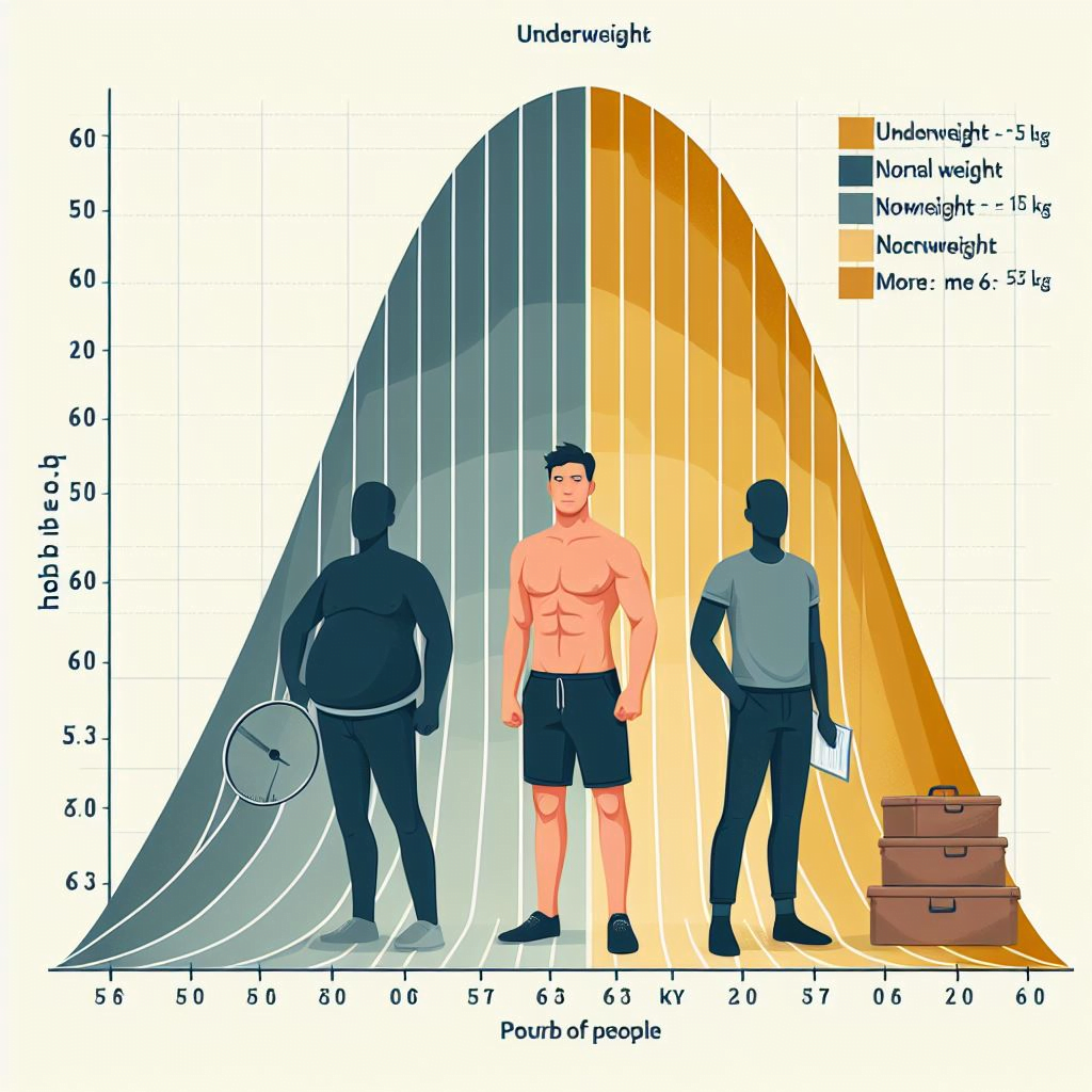
The image shows normal distribution for weight data where, here in this data mean is 60 kg standard deviation is 15 kg and we are trying to find out.
- What is the probability that people weigh less than 55 kg?
- What is the probability that people weigh more than 75 kg?
- What is the probability that people weigh between 58 kg to 70 kg?
For this example, we assume that random variable weight of people follows a normal distribution.
Watch the video to understand calculation
What is a Random Variable?
Random variable is a variable whose value depends on outcome of a random event.
Types of Random Variables
Discrete Random Variables
They have countable number of values to be picked from, it is like picking one value from a set of values. they often have fixed gaps between the values. for example, rolling a dice, there are 6 possible values with fixed interval between them. you cannot 2.5 in rolling a dice. it is going to be eighter 2 or 3.
Continuous Random Variables
They can have any value within a certain range, and the number of possible outcomes are infinite, for example, measuring temperature.
We hope you found the information helpful! If you learned something valuable, consider sharing it with your friends, family, and social networks.
Also Read:
- Understanding Probability
- Understanding Population Variance
- Central Tendency: Sample Mean and Population Mean
- Difference between percentage and percentile
Hi, I am Vishal Jaiswal, I have about a decade of experience of working in MNCs like Genpact, Savista, Ingenious. Currently i am working in EXL as a senior quality analyst. Using my writing skills i want to share the experience i have gained and help as many as i can.