

What is Chi-Square test?
The chi-square test (χ²) is a non-parametric statistical test used to analyze categorical data. It helps determine whether the observed frequencies of a variable (e.g., the number of people in different categories) differ significantly from what would be expected based on a specific hypothesis.
Here’s a breakdown of the chi-square test:
What it does:
- Compares observed frequencies in one or more categories with expected frequencies.
- Assesses the relationship between two categorical variables (e.g., testing if gender and political affiliation are related).
- Evaluates how well a sample distribution fits a theoretical distribution (e.g., testing if coin flips are fair).
Requirements:
- Categorical Data: The data must be categorical, meaning it consists of distinct categories or groups (e.g., hair color, political party affiliation).
- Minimum Expected Frequencies: Each category should have a minimum expected frequency (usually 5 or more) to ensure the test’s validity.
- Independence of Observations: Data points should be independent, meaning the selection of one observation doesn’t influence the selection of another.
Steps to Conduct a Chi-Square Test:
- Define your hypothesis:
- Null Hypothesis (H₀): There is no significant difference between the observed and expected frequencies.
- Alternative Hypothesis (H₁): There is a significant difference between the observed and expected frequencies.
- Create a contingency table: This table shows the observed and expected frequencies for each category.
- Calculate the chi-square statistic (χ²):
- Formula:
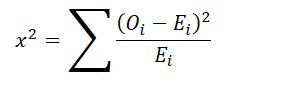
- Where:
- χ²: Chi-square statistic
- Σ: Summation operator (sum over all categories)
- Oi: Observed frequency for category i
- Ei: Expected frequency for category i
- Where:
- Formula:
- Determine the degrees of freedom (df):
- Formula: df = (rows – 1) x (columns – 1)
- Where:
- df: Degrees of freedom
- rows: Number of rows in the contingency table
- columns: Number of columns in the contingency table
- Where:
- Formula: df = (rows – 1) x (columns – 1)
- Find the critical chi-square value: This value is obtained from a chi-square distribution table based on the degrees of freedom and chosen significance level (e.g., 0.05).
- Compare the chi-square statistic to the critical value:
- If the chi-square statistic is greater than the critical value, you reject the null hypothesis (H₀). This suggests a statistically significant difference between observed and expected frequencies.
- If the chi-square statistic is less than or equal to the critical value, you fail to reject the null hypothesis (H₀). There’s not enough evidence to claim a significant difference.
- Interpret the results:
- A rejected null hypothesis suggests a significant difference, but it doesn’t tell you the direction or strength of the difference.
- Consider the magnitude of the chi-square statistic and the context of your research question for a more comprehensive interpretation.
Types of Chi-Square Tests:
- Chi-Square Goodness-of-Fit Test: Tests if the observed frequency distribution of a single categorical variable matches a specific theoretical distribution.
- Chi-Square Test of Independence: Tests if two categorical variables are statistically independent (not related).
Remember: Statistical software can automate most of these calculations, making the chi-square test easier to perform.
Example Calculation of Chi-Square Test
Scenario: We want to test if the color preference of children is independent of their gender. We surveyed a group of 100 children and asked them their favorite color (red, blue, or green) and their gender (boy or girl).
Step 1: Create a Contingency Table:
| Color | Boy | Girl | Total |
|---|---|---|---|
| Red | 20 | 15 | 35 |
| Blue | 25 | 20 | 45 |
| Green | 10 | 25 | 35 |
| Total | 55 | 60 | 100 |
Step 2: Calculate Expected Frequencies:
The expected frequency for each cell is calculated by multiplying the row and column totals and dividing by the grand total (100).
| Color | Boy | Girl | Total |
|---|---|---|---|
| Red | (55 * 35) / 100 = 19.25 | (60 * 35) / 100 = 15.75 | 35 |
| Blue | (55 * 45) / 100 = 24.75 | (60 * 45) / 100 = 20.25 | 45 |
| Green | (55 * 35) / 100 = 19.25 | (60 * 35) / 100 = 15.75 | 35 |
| Total | 55 | 60 | 100 |
Step 3: Calculate Chi-Square Statistic:
For each cell, subtract the observed frequency (Oi) from the expected frequency (Ei), square the difference, and then divide by the expected frequency. Finally, sum all these values to get the chi-square statistic (χ²).
| Color | Boy | Girl | (Oi – Ei)² | (Oi – Ei)² / Ei |
|---|---|---|---|---|
| Red | 20 – 19.25 | 15 – 15.75 | 0.0625 | 0.0032 |
| Blue | 25 – 24.75 | 20 – 20.25 | 0.0625 | 0.0025 |
| Green | 10 – 19.25 | 25 – 15.75 | 84.64 | 4.36 |
| Total | 4.6877 |
Step 4: Determine Degrees of Freedom:
df = (rows – 1) * (columns – 1) = (3 – 1) * (2 – 1) = 2
Step 5: Find the Critical Chi-Square Value:
Using a chi-square distribution table with 2 degrees of freedom and a significance level of 0.05 (α = 0.05), the critical chi-square value is 5.991.
Step 6: Compare Chi-Square Statistic to Critical Value:
Our calculated chi-square statistic (4.6877) is less than the critical value (5.991).
Step 7: Interpret the Results:
Since the chi-square statistic is less than the critical value, we fail to reject the null hypothesis (H₀). This means there is not enough evidence to conclude that the color preference of children is dependent on their gender.
Note: This is a simplified example. In real-world scenarios, you would use statistical software to perform the calculations and obtain a p-value to assess the statistical significance of the results.
We hope you found the information helpful! If you learned something valuable, consider sharing it with your friends, family, and social networks.
Also Read:
- Mann-Whitney U Test Explained
- Chi-Square Test Explained
- ANOVA Analysis of Variance Explained
- T-Test Explained
- Z-Test Explained
- Wilcoxon Signed-Rank Test Explained
Hi, I am Vishal Jaiswal, I have about a decade of experience of working in MNCs like Genpact, Savista, Ingenious. Currently i am working in EXL as a senior quality analyst. Using my writing skills i want to share the experience i have gained and help as many as i can.